Cockcroft Headroom Plot - Part 2 - R Version

I kept tweaking the code, and came up with a prettier version, that also has a small time series view of the throughput in the top right corner.



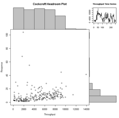
The code for this is

chp <- function(x,y,xl="Throughput",yl="Response",tl="Throughput Time Series", ml="Cockcroft Headroom Plot") {
       xhist <- hist(x,plot=FALSE)
       yhist <- hist(y, plot=FALSE)
       xrange <- c(0,max(x))
       yrange <- c(0,max(y))
       nf <- layout(matrix(c(2,4,1,3),2,2,byrow=TRUE), c(3,1), c(1,3), TRUE)
       layout.show(nf)
       par(mar=c(5,4,0,0))
       plot(x, y, xlim=xrange, ylim=yrange, xlab=xl, ylab=yl)
       par(mar=c(0,4,3,0))
       barplot(xhist$counts, axes=FALSE, ylim=c(0, max(xhist$counts)), space=0, main=ml)
       par(mar=c(5,0,0,1))
       barplot(yhist$counts, axes=FALSE, xlim=c(0,max(yhist$counts)), space=0, horiz=TRUE)
       par(mar=c(2.5,1.5,3,1))
       plot(x, main=tl, cex.axis=0.8, cex.main=0.8, type="S")
}

I also made a wrapper function that steps through the data over time in chunks.

> chp.step <- function(x, y, steps=10, secs=1.0) {
    xl <- length(x)
    step <- xl/steps
    for(n in 0:(steps-1)) {
        Sys.sleep(secs)
        chp(x[(1+n*step):min((n+1)*step,xl)],y[(1+n*step):min((n+1)*step,xl)])
    }
}

To run this smoothly on windows, I had to disable double buffering using

> options("windowsBuffered"=FALSE)

and close the graphics window so that a new one opens with the new option.

The data is displayed using the same calls as described in Part 1. The next step is to try some different data sets and work on detecting saturation automatically.